Algorithmic Complexity

Introduction

Algorithmic complexity is concerned about how fast or slow particular algorithm performs. We define complexity as a numerical function T(n) - time versus the input size n. We want to define time taken by an algorithm without depending on the implementation details. But you agree that T(n) does depend on the implementation! A given algorithm will take different amounts of time on the same inputs depending on such factors as: processor speed; instruction set, disk speed, brand of compiler and etc. The way around is to estimate efficiency of each algorithm asymptotically. We will measure time T(n) as the number of elementary "steps" (defined in any way), provided each such step takes constant time.
Let us consider two classical examples: addition of two integers. We will add two integers digit by digit (or bit by bit), and this will define a "step" in our computational model. Therefore, we say that addition of two n-bit integers takes n steps. Consequently, the total computational time is T(n) = c * n, where c is time taken by addition of two bits. On different computers, additon of two bits might take different time, say c₁ and c₂, thus the additon of two n-bit integers takes T(n) = c₁ * n and T(n) = c₂* n respectively. This shows that different machines result in different slopes, but time T(n) grows linearly as input size increases.
The process of abstracting away details and determining the rate of resource usage in terms of the input size is one of the fundamental ideas in computer science.

Asymptotic Notations

The goal of computational complexity is to classify algorithms according to their performances. We will represent the time function T(n) using the "big-O" notation to express an algorithm runtime complexity. For example, the following statement

T(n) = O(n²) says that an algorithm has a quadratic time complexity.

Definition of "big Oh"

For any monotonic functions f(n) and g(n) from the positive integers to the positive integers, we say that f(n) = O(g(n)) when there exist constants c > 0 and n₀ > 0 such that
f(n) ≤ c * g(n), for all n ≥ n₀ Intuitively, this means that function f(n) does not grow faster than g(n), or that function g(n) is an upper bound for f(n), for all sufficiently large n→∞
Here is a graphic representation of f(n) = O(g(n)) relation:
Examples:

• 1 = O(n)
• n = O(n²)
• log(n) = O(n)
• 2 n + 1 = O(n)

The "big-O" notation is not symmetric: n = O(n²) but n² ≠ O(n).
Exercise. Let us prove n² + 2 n + 1 = O(n²). We must find such c and n₀ that n ² + 2 n + 1 ≤ c*n². Let n₀=1, then for n ≥ 1
1 + 2 n + n² ≤ n + 2 n + n² ≤ n² + 2 n² + n ² = 4 n² Therefore, c = 4.

Constant Time: O(1)

An algorithm is said to run in constant time if it requires the same amount of time regardless of the input size. Examples:

• array: accessing any element
• fixed-size stack: push and pop methods
• fixed-size queue: enqueue and dequeue methods

Linear Time: O(n)

An algorithm is said to run in linear time if its time execution is directly proportional to the input size, i.e. time grows linearly as input size increases. Examples:

• array: linear search, traversing, find minimum
• ArrayList: contains method
• queue: contains method

Logarithmic Time: O(log n)

An algorithm is said to run in logarithmic time if its time execution is proportional to the logarithm of the input size. Example:

• binary search

Recall the "twenty questions" game - the task is to guess the value of a hidden number in an interval. Each time you make a guess, you are told whether your guess iss too high or too low. Twenty questions game imploies a strategy that uses your guess number to halve the interval size. This is an example of the general problem-solving method known as binary search locate the element a in a sorted (in ascending order) array by first comparing a with the middle element and then (if they are not equal) dividing the array into two subarrays; if a is less than the middle element you repeat the whole procedure in the left subarray, otherwise - in the right subarray. The procedure repeats until a is found or subarray is a zero dimension.

Note, log(n) < n, when n→∞. Algorithms that run in O(log n) does not use the whole input.

Quadratic Time: O(n²)

An algorithm is said to run in logarithmic time if its time execution is proportional to the square of the input size. Examples:

• bubble sort, selection sort, insertion sort

Definition of "big Omega"

We need the notation for the lower bound. A capital omega Ω notation is used in this case. We say that f(n) = Ω(g(n)) when there exist constant c that f(n) ≥ c*g(n) for for all sufficiently large n. Examples

• n = Ω(1)
• n² = Ω(n)
• n² = Ω(n log(n))
• 2 n + 1 = O(n)

Definition of "big Theta"

To measure the complexity of a particular algorithm, means to find the upper and lower bounds. A new notation is used in this case. We say that f(n) = Θ(g(n)) if and only f(n) = O(g(n)) and f(n) = Ω(g(n)). Examples

• 2 n = Θ(n)
• n² + 2 n + 1 = Θ( n²)

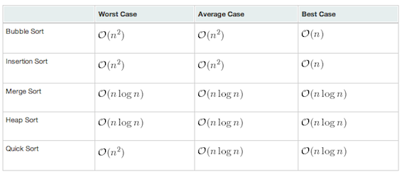
Analysis of Algorithms

The term analysis of algorithms is used to describe approaches to the study of the performance of algorithms. In this course we will perform the following types of analysis:

• the worst-case runtime complexity of the algorithm is the function defined by the maximum number of steps taken on any instance of size a.
• the best-case runtime complexity of the algorithm is the function defined by the minimum number of steps taken on any instance of size a.
• the average case runtime complexity of the algorithm is the function defined by an average number of steps taken on any instance of size a.
• the amortized runtime complexity of the algorithm is the function defined by a sequence of operations applied to the input of size a and averaged over time.

Example. Let us consider an algorithm of sequential searching in an array.of size n.

Its worst-case runtime complexity is O(n)
Its best-case runtime complexity is O(1)
Its average case runtime complexity is O(n/2)=O(n)

Amortized Time Complexity

Consider a dynamic array stack. In this model push() will double up the array size if there is no enough space. Since copying arrays cannot be performed in constant time, we say that push is also cannot be done in constant time. In this section, we will show that push() takes amortized constant time.
Let us count the number of copying operations needed to do a sequence of pushes.

push()	copy	old array size	new array size
1	0	1	-
2	1	1	2
3	2	2	4
4	0	4	-
5	4	4	8
6	0	8	-
7	0	8	-
8	0	8	-
9	8	8	16

We see that 3 pushes requires 2 + 1 = 3 copies.
We see that 5 pushes requires 4 + 2 + 1 = 7 copies.
We see that 9 pushes requires 8 + 4 + 2 + 1 = 15 copies.
In general, 2ⁿ+1 pushes requires 2ⁿ + 2^n-1+ ... + 2 + 1 = 2ⁿ⁺¹ - 1 copies.
Asymptotically speaking, the number of copies is about the same as the number of pushes.

       2n+1 - 1
limit --------- = 2 = O(1)
 n→∞   2n + 1

We say that the algorithm runs at amortized constant time.